The story behind the migration from Greenplum data warehouse to Google BigQuery. Written about the migration steps, assessments, data export, common challenges and its solution.

Greenplum is a popular opensource data warehouse software. It is built on top of the PostgreSQL database(which is my favorite database). It supports MPP architecture and columnar storage for petabyte-scale processing. You can run federated queries including Hadoop, Cloud Storage, ORC, AVRO, Parquet, and other Polyglot data stores. Hit here to learn more about it.

On-Prem Architecture: #

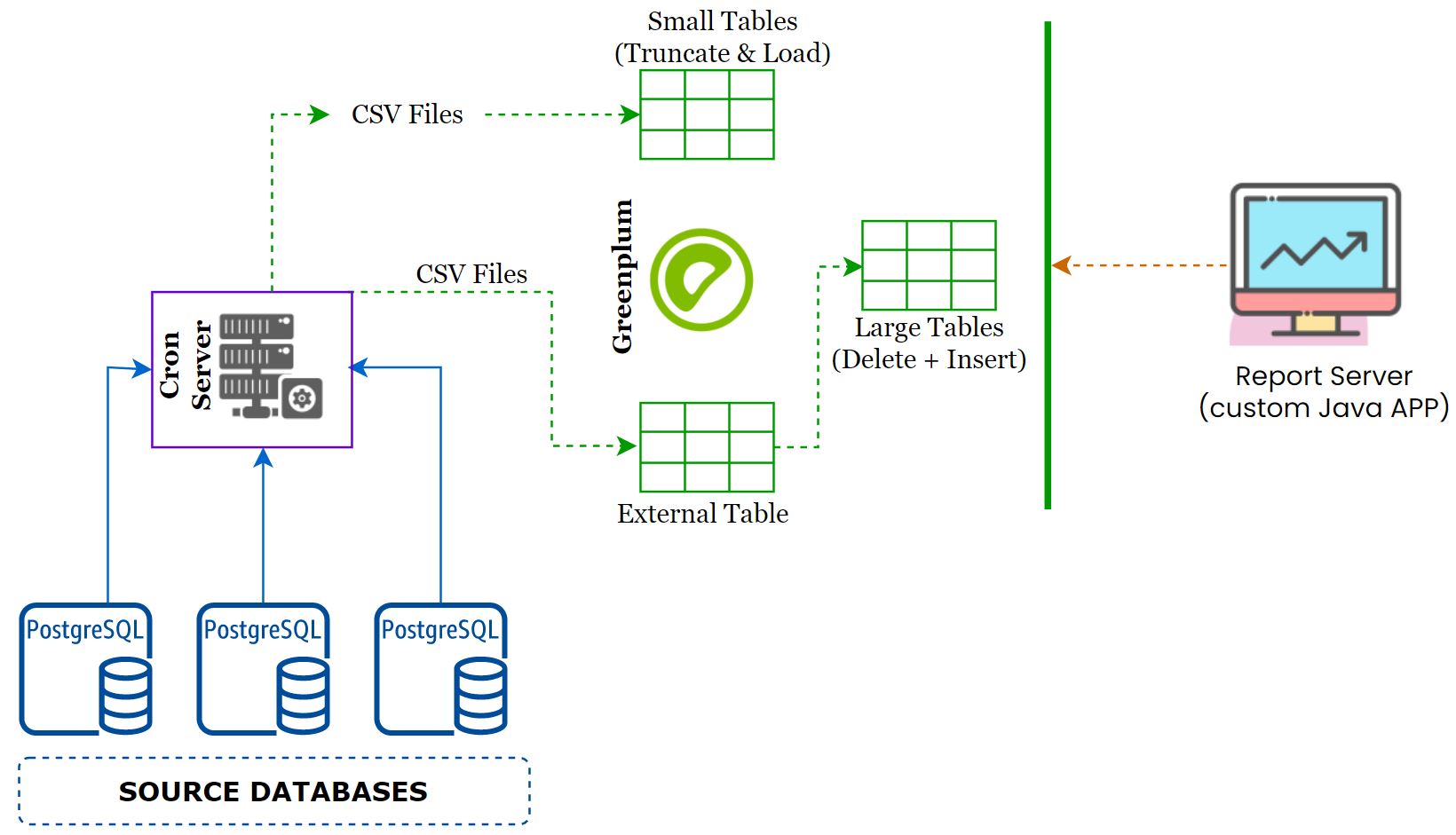
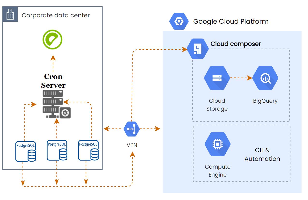
• The customer had a single giant Greenplum server which is their main data warehouse.
• They were collecting the data from 10+ PostgreSQL servers and push it into the Greenplum with near real-time sync.
• The data sync job had been written in shell scripts and deployed on a dedicated cron server.
• Some of the tables were huge and they did partition on an integer column.
• The total uncompressed size of the Greenplum database is 15TB.
• A java based reporting tool developed by the customer was used for visualizing.
• An opensource tool(forgot the name) used to schedule the reports - A flat file will be sent via email.

Pain with the Greenplum: #

It’s an amazing database, no doubt about it. But when it’s coming to operations, there are more pain points with the existing Greenplum setup.

• Single node monster - Even though it’s a huge one, it had a single point of failure.
• Workload management - There is no workload management implemented which lets everyone run any queries.
• Incorrect Partition - 80% of the data was on a single partition, while creating the partition, they manually added a column that refers to the partition number, and using the same number for all the data sync jobs caused more data on a single partition.
• Index - Some indices on the large tables consumed more space.
• Vaccum - If you are coming from a PostgreSQL background, then you know the pain of running a vacuum process.
• Hardware limitation - There are a lot of constraints when coming to add more hardware to the existing cluster. So more restrictions on adding a few more nodes, dedicated storage for database snapshots and its retention, and many more limitations.
• Backup & DR - Performing a logical backup on a 15TB database is not a simple process also DR setup with continuous backup for the point-in-time recovery is another headache.

BigQuery - The Beast: #

Im not going to write about the BigQuery here, everyone knows this Beast. But a few features,

• Map-Reduce and columnar processing.
• Cheap storage cost.
• Serverless and no limitation on the number of CPU cores and memory(but slots are there)
• No Index, No Vaccum, No Backup, No HA, No DR

Solution Overview: #

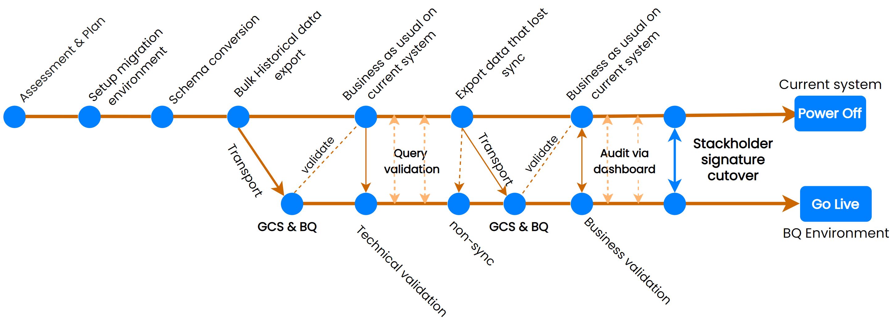
Assess migration tasks

• Understand the scope
• Identify the objects for the migration

Setup migration environment

• A VM with client tools to access the Greenplum server and script the entire migration

Migrate - Dev environment

• Convert the schema (tables)
• Create tables on BigQuery
• Convert any UDF or Procedure
• Export historical data to Google Cloud Storage and import into BigQuery
• Export incremental Data and Catch up with Greenplum
• Migrate the Shell Scripts to Airflow DAGs for data pipeline
• Validate data
• Business validation (including optional dual-running)
• Implement monitoring
• Cutover

Migrate - PROD environment

• Convert the schema (tables)
• Create tables on BigQuery
• Convert any UDF or Procedure
• Export historical data to Google Cloud Storage and import into BigQuery
• Export incremental Data and Catch up with Greenplum
• Migrate the Shell Scripts to Airflow DAGs for data pipeline
• Validate data
• Business validation (including optional dual-running)
• Implement monitoring
• Cutover

Assessment: #

For the initial few days, we spent most of your time on the assessment part to understand better the current system(table structure, and process). Here are our Assessment categories.

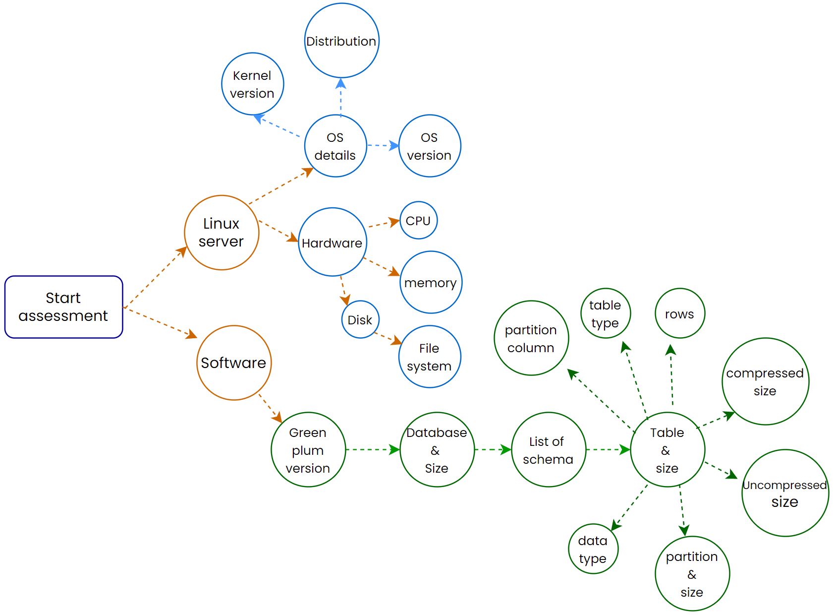
The assessment scripts(for Greenplum) are available in my GitHub Repo

Setting up Migration Environment: #

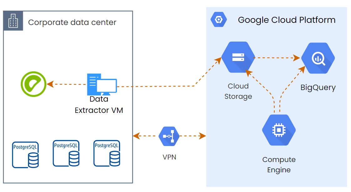
We had to run some SQL queries and Python scripts to do the assessment and the data export. So we provisioned a VM on the On-Prem side with a large disk to stage the data before uploading it to GCS(but later we removed it, continue reading to know why) and another VM on the GCP side to import the GCS data to BQ and run some BQ automation scripts. A VPN connection is already established between GCP and the On-prem data center.

Schema Conversion (tables): #

This is the most important part, if we didn’t use the proper data type or partition then we have to do everything one more time. There are so many tables that we want to convert its schema to BigQuery. Manually creating all of them will be a difficult task.

We were using airflow for all the data orchestration, so we deployed a DAG that will do the DDL migration.

We created a python function to extract the tables, columns, and their data type from the information_schema and map the BigQuery equivalent data type. Then it’ll generate the BigQuery schema file.

The complete airflow dag is available here

Note: The data types are mapped with almost correct BQ data type, if you want to change, then you can change it. Some data types won’t support BQ, so it’ll convert them to STRING.

Pro Tip

If your tables are properly partitioned on Greenplum, and want to migrate the same partition structure, then we have another airflow DAG for this. This will understand the partition structure and migrate the complete table with proper data type and partition. But it won’t support STRING partition columns. Read More from my previous blog and get the DAG.

Historical data migration: #

This is the part where I spent more of the time. Initially, I thought it’s just a COPY command, then upload it to GCS and then import it to BQ. So simple right? But it was not that smooth.

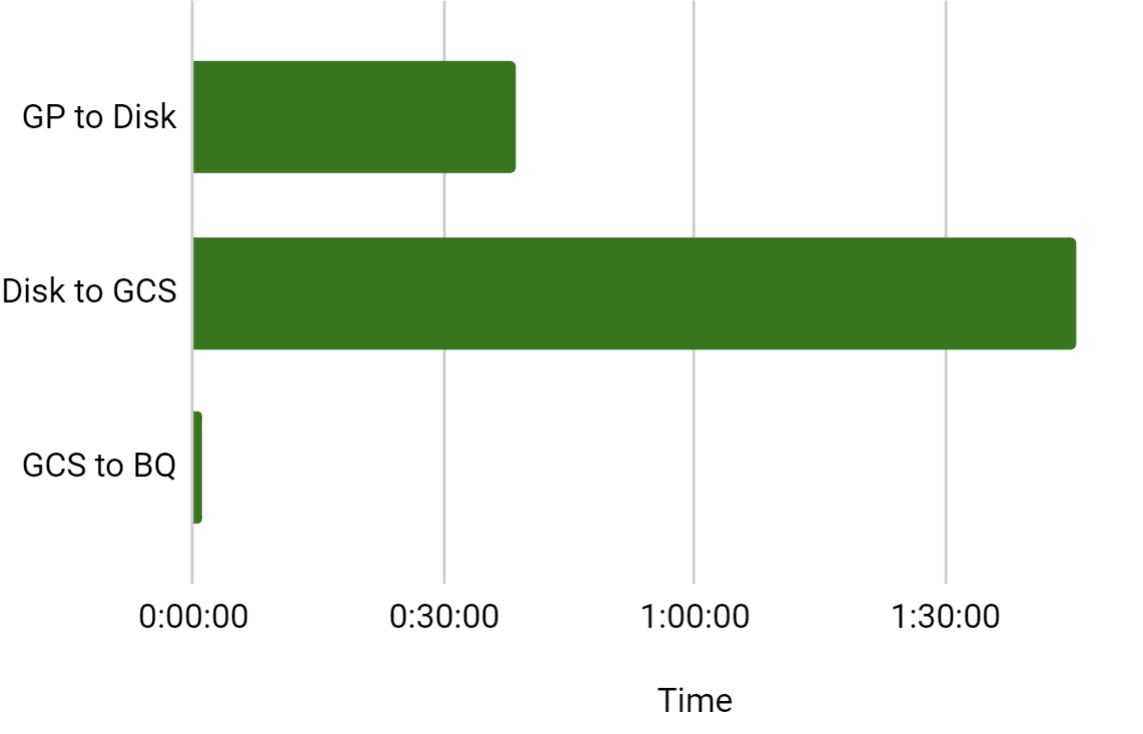
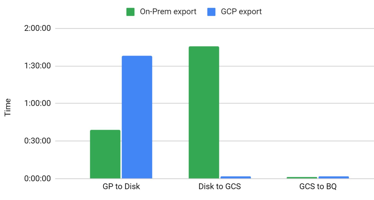
Export from On-Prem: #

Unfortunately, we only had VPN, not the partner interconnect. So I thought to extract the data from the table to a VM which is on the same data center, this will improve the export performance. Then export that files to GCS. Some tables were huge(5TB) and belong to the same partition. We attached 2TB HDD to export the VM.

Problem #1 Network Bandwidth: #

Export using COPY select * from won’t be the right choice. So I wanted to try the whole process with a small chunk of data. On the given table I took a timestamp column for the chunk and exported the data for 30days. Not bad. Then started exporting the data to GCS. Here the actual problem started. It took 1hr and 45mins. This is the worst part of the migration.

gcloud cli output:

[1/1 files][169.5 GiB] 100% Done 26.3 MiB/s ETA 00:00:00
Operation completed over 1 objects/169.5 GiB.

Solution

The reason why we had to use the on-prem server to export the data is to reduce the latency during the COPY operation. But transfer speed is too bad due to low bandwidth. So we tried to export the data from Greenplum to a stage VM which is provisioned on the GCP side. It had both pros & cons. The Copy operation took 01:38:00 but luckily the export process from VM to GCS is too quick. It’s just 2mins. Import to BQ from GCS is not having much difference.

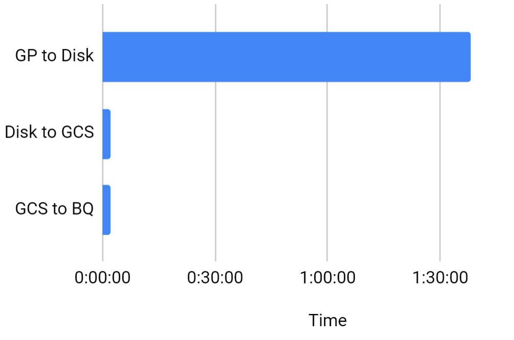
Due to VPN latency, the export from GP took more time, but overall it reduced the time by 1.5Hr.

Problem #2 CSV files are large in size #

When I do the export for a single month, the output file size was 165GB. While importing into BigQuery, If it throws an error, then finding the problematic row will be very difficult with a large file. In the Greenplum COPY command, it’s not possible to chunk it. I tried to check any python modules like psycopg

Solution:

Finally, I decided to go with the shell script to extract the data and split the files into small chunks based on the number of rows using the SPLIT command. Here is the sample snippet.

psql -U bhuvanesh -h YOUR_GP_IP -d database  -c "COPY (SELECT * FROM myschema.table ) TO stdout WITH  DELIMITER '|' CSV ;" | split  -a3 -dl 1000000 --filter='gzip > $FILE.gz' - /export/data/table/table.csv_

Note: While using the split command, don’t mention the file size, because it’ll break a single row into two different files.

Here is my full script for extracting the table for the last 4 years month-wise and upload it to GCS.

Problem #3 JSON Data #

Some of the tables had a TEXT data type column where the customer stored JSON response inside it. I understood this will break the data load and throw errors related to delimiter and quotes. Greenplum has an option to add a proper quote in the COPY command. But the version of Greenplum won’t support wildcard for columns to add a quote. We had to manually pass all the column names that need to be quoted.

Solution:

It’s not a big deal, I just ran a query to find all string columns from the Information_schema.columns and used that output in my COPY command with FORCE QUOTE option

select
   string_agg(column_name, ',' 
order by
   ordinal_position) 
from
   information_schema.columns 
where
   table_schema = 'myschema' 
   and table_name = 'table' 
   and data_type = 'character varying';

If you want to add quotes for col1,col2, and col3 then use the following command.

psql -U bhuvanesh -h YOUR_GP_IP -d database  -c "COPY (SELECT * FROM myschema.table ) TO stdout WITH  DELIMITER '|' CSV  FORCE QUOTE col1,col2,col3;" | split  -a3 -dl 1000000 --filter='gzip > $FILE.gz' - /export/data/table/table.csv_

Problem #4 New Line Character(\n) with Split Command #

This is not a new problem for data engineers. If the row contains the new line character, then the next line will be considered for the next row. But in BigQuery we can easily solve it by adding a flag –allow_quoted_newlines. But while using the split command it gave me problems. I was splitting by 1000000 lines. If the 1000000’th line has any new line character, then the values after the \n will move to the next file.

Example

id, name, address, email
1, "my name","house name, street \n
city, state, PIN", "[email protected]"

If this line will be the last line then file1 will end with

1, "my name","house name, street \n

File2 will start with

city, state, PIN", "[email protected]"

So File1’s last line and File2’s first line will break the data load.

Solution:

We can’t solve this in the SPLIT command, so we have to deal with this at the database level. So in the COPY command, we used the replace function to remove the new line characters.

psql -U bhuvanesh -h YOUR_GP_IP -d database -c "COPY (select col1,col2,col3,replace(col4,E'\n','' ) as col4,col5 FROM myschema.table) TO stdout WITH  DELIMITER '|' CSV FORCE QUOTE col1,col2,col3;" | split  -a3 -dl 10000000 --filter='gzip > $FILE.gz' - /export/data/table/table.csv_   

Bonus Tip - Alternate to Split: #

Sometimes we want to keep the newline characters to keep the exact format. But the SPLIT command will break the row. But there is an alternate way that you can generate the export command only for X number of rows. But a SERIAL column(Primary key column) must be there on your tables.

Example

Export 1000 rows as the chunk.

• Min value on the table - 1
• Max value on the table - 12000 If we want to export with 1000 chunks, then the first export should COPY like below.

select  * from table where id between 1 and 1000;

And then 2nd iteration will be 1001 to 2000

select  * from table where id between 1001 and 2000;

Use the following SQL command to generate the IDs with 1000 intervals(basically, the where condition).

psql -U bhuvanesh -h YOUR_GP_IP -d database -t -c"select
(min((Primary_KEY_Column - 1) / 1000) * 1000 + 1) || ' and ' || (min((Primary_KEY_Column - 1) / 1000) * 1000 + 1000) as id 
from
   schema.table1 
group by
(Primary_KEY_Column - 1) / 1000 
order by
(Primary_KEY_Column - 1) / 1000" > chunk_id_table1

Then use the following shell script to pick the IDs from the output of the above SQL query and create a loop to pass the ID(where condition) one by one.

#/bin/bash
chunk=1
while read -r i
do

psql -U bhuvanesh -h YOUR_GP_IP -d database  -c "COPY (SELECT * FROM myschema.table WHERE id between $i  ) TO '/export/data/mytable/file_$chunk.csv' WITH  DELIMITER '|' CSV  FORCE QUOTE col1,col2,col3;" 

# Export to GCS
gsutil -m rsync /export/data/mytable/ gs://export/prod-data/mytable/

chunk=`expr $chunk + 1`
done < chunk_id_table1

After solving these things, finally, the historical data got imported into the BigQuery tables. But remember these points when you load the data from GCS.

1. If you use the wildcard parameter(gs://bucket/folder/*.csv) to load all the files inside a folder, then make sure only 10k files inside it. allow-jagged-rows not always a good option.
2. bq load CLI command will return up to 5 problematic files in case if it has bad records. It doesn’t mean that only 5 files have the issue.
3. Always use max-bad-records=0 because we don’t want to lose any single row.
4. Don’t include the column names in the CSV file if you are splitting into small chunks. Because the first file needs to skip the header and the rest of the files should not. So while importing if you mention skip rows then 1st row of every file will be skipped(if use wildcard)

Historical load Validation #

We export the data with split command and each file contains 1000000 rows. So we calculated the total rows exported based on the number of output files.

Note: My file naming conversion is file.0001.csv.gz So to find the last file, we need to remove the file. and .csv.gz string. Also, there is no guarantee that the last file also having the same number of rows, so we have to manually check the lines for the last file. (see the script below, and feel free to modify as per your naming conversion)

Use the script to find the total exported rows.

## No new line characters
## No headers
cd /path/where/files/exported/for/Table-1/
total_files_minus_1=$(($(ls |wc -l) - 1))
last_file=$(ls | sed 's/file.//g'|sed 's/.csv.gz//g'|sort -n -r |head -n 1)
lines_per_file=1000000
lines_in_lastfile=$(zcat file.$last_file.csv.gz | wc -l)
echo $(( $total_files_minus_1 * $lines_per_file + $lines_in_lastfile ))

Now match this number with BigQuery tables.

SELECT Count(*) 
FROM   `bqdataset.tablename`; 

Incremental Load #

The historical load took more than 15days. For catching up on the existing Greenplum, we used two different methods. Some tables are not transaction heavy and there is no archival on the source databases. So we can directly fetch the incremental data based on the timestamp column.

Some tables are really heavy in the transaction and delete the records that are older than 2 days(based on some conditions), for those tables, we exported the last 13 days of data from the Greenplum and push it to GCS then imported it to BigQuery. After that, the remaining 2 days of data are exported directly from the source databases.

Migrate Data pipeline from Shell scripts to Airflow: #

This is another major scope of this migration, all the shell scripts got replaced by Google cloud composer(managed airflow). They had some UDF for the data load. Since we moved everything to Airflow, so we don’t need these to be migrated to BigQuery.

The pipeline use case is very simple.

• 30% of the tables are small in size and truncate and load would be preferred by the customer with 1Hr interval.
• 40% of the tables are in a decent size, and they had a 2mins sync interval based on the timestamp value for the incremental load.
• The remaining 30% of the tables are super large tables and transaction heavy and they had a 1min sync interval. This is also based on the timestamp value for the incremental load.

Developing the airflow DAGs is easy, but using the same strategy as like on-prem was a bad idea. Refer the on-prem architecture to understand the data pipeline.

We let the shell script sync the data to Greenplum and deployed the Airflow for BQ data sync.

I’ll publish one more blog post about these airflow dags with Dynamic DAG and task generation.

Problem #5 BigQuery Merge #

The existing pipeline for the incremental sync did the DELETE + INSERT based on the primary key column. Initially, we tried the same approach with the merge statement for the small tables and it worked. But when we checked this on the super large tables(just only 1 try) where some tables are in 3TB, 2TB, it affects the execution time(it took a bit longer than expected). BigQuery is a columnar format storage system and MERGE means it should talk to all the columns irrespective of how many rows that you are updating. So every 2mins, if we read 3TB of the data then think about the cost, it’ll be too much and it’s a bad solution.

Solution

We don’t want to update everything on each sync. So we just made the data import as append-only. Then created a view on top of the table to de-dup the data.

WITH
  CTE AS (
  SELECT
    *,
    ROW_NUMBER() OVER (PARTITION BY pk_column ORDER BY update_timestamp DESC ) RowNumber
  FROM
    `myschema.table1`)
SELECT
  *
FROM
  CTE
WHERE
  RowNumber =1

Problem #6 Incremental Load Cost - Fetch timestamp from BQ table #

For the 1min and 2mins sync, jobs need to find the max timestamp value from the BQ table then it’ll fetch the data from the source table. I was thinking it’s just one single column and it won’t make much cost difference. But my assumption was wrong. Fetching the column every 2mins and a few large tables ended up with $1.5k per day.

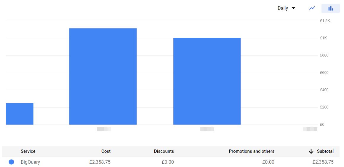
Solution

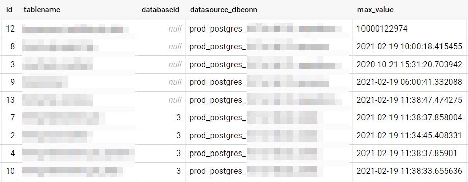
There is no way to solve this with the existing pipeline, so I have changed the data pipeline logic with a metatable where it’ll maintain the max time value for all the tables. So the fetch max(timestamp) step will get the timestamp value from this table and update the new value at the end of the pipeline. Some tables will use the ID column as the max value identifier instead of timestamp, so the same metatable helped to store that value as well.

-- databaseid and datasource_dbconn is used in our use case
-- you can skip those columns
CREATE TABLE
  bqdataset.tablemeta (id INT64 NOT NULL,
    tablename STRING NOT NULL,
    datbabaseid INT64,
    datasource_dbconn STRING NOT NULL,
    maxvalue STRING NOT NULL)

This helped us to reduce the billing.

Problem #7 Partition limitation #

For the large tables, we did the partition on a timestamp column and the partition type was DAY. Throughout the day the pipeline was running fine but some batch jobs on the source database made the update on millions of rows for a table. It hits the partition limitation.

https://cloud.google.com/bigquery/quotas#partitioned_tables

BigQuery job failed. Final error was: {'reason': 'quotaExceeded', 'location': 'partition_modifications_per_column_partitioned_table.long', 'message': 'Quota exceeded: Your table exceeded quota for Number of partition modifications to a column partitioned table. For more information, see https://cloud.google.com/bigquery/troubleshooting-errors'}.

Solution

We recreated the table with the partition type as YEAR.

Final Data Validation: #

This is the last step of the testing. We ran multiple iterations of testing to validate the data. The very first level of testing starts with row count. We stopped the data sync on both sides then we started the data validation. Some of the basic metrics are,

• Row count
• Row count by Year, month, day.
• Min and Max ID.
• SUM of some integer column.
• Ran some frequently used KPI queries.
• Random queries.

Do you think was it smooth? actually no.

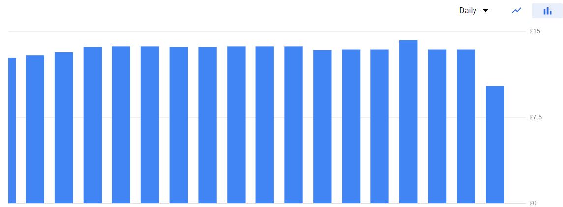
Problem #8 BQ billing surge #

As I mentioned earlier, some of the tables are huge. Running queries frequently on these tables consumed more data scans that ended up with more cost in just one day. Then we were thinking about how to control the cost only during the validation part.

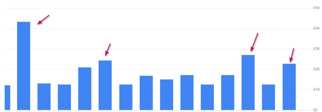
Solution:

Flex slots - Yes, we used flex slots. But in a different method. Instead of purchase the slot at one time, we purchased it when we start our validation and retire the slot when we finished our work for the day. Even if we take a break for more than 30mins, then we retired the slots. We bought 200 slots. This drastically reduced the cost during the validation phase.

Finally, point the dashboard application to the BigQuery and get the reports, and then compared the data between Greenplum and BigQuery.

Note: We tried both the Google BQ driver and the Simba BQ,, driver. But the latest version of the driver is a bit slower than the older version. So please check with a few driver versions.

Conclusion: #

The blog post intends to give you how you can manage the Greenplum to BigQuery. Because I didn’t find any blogs or documentation for this. And some common challenges that you’ll face during the migration. We have done many things to optimize, but those are not relevant to this blog. Happy Migration !!!